第 4 章 数据可视化
4.1 ggplot绘图
4.1.2 中文字体
中文字体问题总是会在时不时出来捣乱。今天就碰到了ggplot2绘图时,latex pdf输出和html网页输出显示不一致的问题(类似的 问题报告)。
google神搜一遍,大家普遍把问题指向:
操作系统OS问题。Linux/Mac OS普遍采用UTF-8编码格式,而Windows系统则坚持GBK编码格式。因此,如果Rstudio里Rmarkdown文件用UTF-8编码,自然就会导致Windowns粉出现悲催的混乱事件。Windowns系统下还可能存在本地字体库不全的问题。
中文字体库问题。除了系统阵营的锅,中文字体本身也会给编码世界带来混乱。其实不单是中文字体,CJK字体库就是专门为了解救中文-日文-韩文字体等东亚语言字体问题的。另外就是,字体库有“真体”(TrueType Collection 字体文件 (.ttc))等字体版本。因此,latex包
\usepackage{xeCJK}渲染时,可能会提示错误(类似报告1;报告2)engine或dev问题。第三个锅就是软件的问题了。其一,bookdown下默认的Latex引擎
pdflatex对Unicode characters支持不好,需要改用xelatex引擎(yihuixie留爪)。其二,绘图装置dev也有小九九类似报告。最关键的是绘图装置可以自己根据需要设定,包括:dev=‘cairo_pdf’;dev=‘pdf’;dev=‘svg’(见友情提示)。
具体解决办法:
(windowns系统)安装缺少的字体库。大概就先去看看”c:/windows/fonts”目录吧!。也可以在R中用package如
"showtext"来安装。——不说这个了,都是泪。latex中设定header.tex的包调用。最重要的
\usepackage{xeCJK},大抵如下:
\usepackage{xeCJK}
%\setCJKmainfont{SimSun}
\setCJKmainfont{宋体}  % 字体可以更换
\setCJKmonofont{simsun.ttc} % for \textsf
\setmainfont{宋体} % 設定英文字型
\setromanfont{Georgia} % 字型
\setmonofont{Courier New}- Rmarkdown中设定engine和dev。这个地方倒是有一个逻辑性的问题我之前一直没有弄清楚。engine设好后(如前,最好用
xelatex引擎),不同输出形式(pdf、html)对绘图转置dev需求是不一样的,因此需要考虑latex_engine和dev所处的环境。这个环境不一样,控制的范围自然就不同,但大概有三个级别:a. yaml区域的全局性- output环境; b. R代码块的文档级设置;c.特定R代码块的设置。
环境1:yaml区域的全局性设置
output:
  bookdown::pdf_document2:
    latex_engine: xelatex
    dev: cairo_pdf
环境2:R代码块的文档级设置
{r global_options,echo=FALSE, message=FALSE}
knitr::opts_chunk$set(fig.align='center', dev="cairo_pdf",
                      echo=FALSE, fig.pos = 'H') #
环境3:特定绘图R代码块环境
{r common-get-sum,echo=FALSE, dev="cairo_pdf", message=FALSE,error=FALSE,warning=F, fig.width=10,fig.height=7,fig.cap="学生累计获得通识课程学分情况"}

ggplot() +
  theme(text=element_text(family="Batang", size=12))
总结起来,最后的问题解决就是:
更改pdf全局性环境的引擎为latex_engine: xelatex。
更改pdf全局性环境里绘图装置为:dev: cairo_pdf。设好后就不要画蛇添足再在环境2或环境3中做额外配置了。因为控制范围是不一样的!html输出默认绘图转置为dev: cairo_pdf
因为字体库问题,还得在绘图R代码块里指定一个能够显示的字体。如
theme(text=element_text(family="Batang", size=12))。
最后,html和pdf显示都一致啦!!
4.1.3 调用当前代码块名
既可以直接调用,马上使用代码块名(如下):
library(knitr)
chunk_name <- knitr::opts_current$get()$label
plot(cars)
print(paste0("The current code chunk name is: ", chunk_name ))[1] "The current code chunk name is: cars"也可以先存储多个代码块名,后面再调取使用(见下):
library(knitr)
ll <- opts_current$get()$label
knit_hooks$set(label_list = function(before, options, envir) {
    if(before) ll <<- c(ll,opts_current$get()$label)
})
#opts_chunk$set(label_list=TRUE)print(paste0("The first code chunk name is: ", ll[[1]]) )[1] "The first code chunk name is: knitr_setup"4.1.4 图片的导出
方法1:通过ggplot2::ggsave()函数,可直接导出为位图:
# save plot
ggplot2::ggsave(filename = "pic/network-french-mps-p0.png",
       plot = p0,
       type = "cairo", # you should use this augument to save time
device = "png")方法2:利用officer包以及rvg包导出xlsx或word文档格式下的可编辑矢量图。
library("techme")
# here is my customed function
techme::gg2xlsx
function (p, dir = "pic/ggsave-xlsx/", num_section = 2, num_fig,
names_chunk)
{
path_out <- paste0(dir, "Figure", num_section, "-", num_fig,
"-", names_chunk, ".xlsx")
doc <- officer::read_xlsx()
doc <- rvg::xl_add_vg(doc, sheet = "Feuil1", code = print(p),
width = 12, height = 7, left = 1, top = 2)
print(doc, target = path_out)
}
<bytecode: 0x000002c8fc4340b8>
<environment: namespace:techme>4.2 结构化数据库
在有些时候需要读取或存取大量数据,这时候结构化数据库的使用可以减少Rstudio的缓存压力,也可以保证工作流数据存取的安全性和可靠性。
4.2.1 增量写入数据表
如下代码展示的是“增量型”写入数据表的一种情形。具体应用案例,比如网页数据爬虫时,持续不断地抓取网页表格,并增量写入到本地数据库table中去。
#install.packages(c("dbplyr", "RSQLite"))
#install.packages("DBI")
library(DBI)
require(dbplyr)
require(RSQLite)

# create directory
dir.create("data/market-xian", showWarnings = FALSE)

# create database file
mydb <- dbConnect(
  RSQLite::SQLite(),
  "data/market-xian/market.db"
  )

# append new data table(with same structure) to exist one
dbWriteTable(mydb, "mydf",tail(mtcars),
             append=TRUE,overwite=FALSE)

# show tables in the data base
dbListTables(mydb)

# show me the table
check_out <- tbl(mydb, "mydf") %>%
  as_tibble()

# disconnect to my database
dbDisconnect(mydb)注意:
tbl(mydb, "mydf")返回的是一个S3类对象tbl_SQLiteConnection,是以list形式保存。因此R环境下需要使用as_tibble()函数进一步得到tibble形式的表格(本地dataframe)。但是在直接与SQL对话时(远程dataframe),实际上也可以不做这样的操作。(参看队长问答)。
4.2.2 保持数据列格式
在Rstudio下的tibble数据表,列变量的格式如果是日期类型date,写入SQL 数据库文件时可能会遇到格式丢失的问题。
例如”2018-12-01” 会变成 17866。
为避免这种问题的发生,需要设置extended_types = T。具体代码见下(可参看队长问答):
# connect to database file
mydb <- dbConnect(RSQLite::SQLite(),
                  "data/case-pollution/ozone.db",
                  extended_types = T) # important
4.3 信息可视化
4.3.1 树形图tree graph(文件结构目录树)
经验法则:a.方法1的操作更为直观。b.在
.Rmd的代码块参数中,设置comment=""。
在介绍文件系统时,往往需要将文件目录关系做树形展示(file system tree)。此时我们可以用到R包data.tree。
方法1:直接列出文件路径的data.frame数据集,然后再print()。
library(data.tree)

path <- c(
    "master-SEM/mycss/my-custom-for-video-roomy.css",
    "master-SEM/slide-chn-part1/part00-slide-intro.Rmd",
    "master-SEM/slide-chn-part1/part00-slide-intro.html",
    "master-SEM/slide-chn-part1/part00-slide-intro_files" )

mytree <- data.tree::as.Node(data.frame(pathString = path))

print(mytree)
levelName
1 master-SEM
2 ¦--mycss
3 ¦ °--my-custom-for-video-roomy.css
4 °--slide-chn-part1
5 ¦--part00-slide-intro.Rmd
6 ¦--part00-slide-intro.html
7 °--part00-slide-intro_files 方法2:手动编写目录文件关系的list数据集,然后再直接print()。
library(data.tree)

netlify <- Node$new("netlify")
  static <- netlify$AddChild("static")
    statistics <- static$AddChild("course-advanced-statistics")
    econometrics <- static$AddChild("course-econometrics")
      data <- econometrics$AddChild("data")
      pic <- econometrics$AddChild("pic")
        pic1 <- pic$AddChild("chpt1-log.png")
        pic2 <- pic$AddChild("chpt2-reg.png")
      reading <- econometrics$AddChild("reading")
        files <- reading$AddChild("cht01-history.files")
        html <- reading$AddChild("cht01-history.html")
      intro <- econometrics$AddChild("01-introduction-slide.html")
      reg <- econometrics$AddChild("02-simple-reg-basic-slide.html")
  content <- netlify$AddChild("content")
  public <- netlify$AddChild("public")
  config <- netlify$AddChild("config")
  proj <- netlify$AddChild("netlify.Rproj")

print(netlify)
levelName
1 netlify
2 ¦--static
3 ¦ ¦--course-advanced-statistics
4 ¦ °--course-econometrics
5 ¦ ¦--data
6 ¦ ¦--pic
7 ¦ ¦ ¦--chpt1-log.png
8 ¦ ¦ °--chpt2-reg.png
9 ¦ ¦--reading
10 ¦ ¦ ¦--cht01-history.files
11 ¦ ¦ °--cht01-history.html
12 ¦ ¦--01-introduction-slide.html
13 ¦ °--02-simple-reg-basic-slide.html
14 ¦--content
15 ¦--public
16 ¦--config
17 °--netlify.Rproj 4.3.2 流程图flowchart
流程图(flow chart)常用于编程逻辑过程说明演示。
实现流程图绘制的主要工具包包括:
R包
rstudio/nomnoml(gihub仓库)。优点:独立制图语言(sassy UML diagrams),基于nomnoml.js(演示文档),可绘制复杂的定制化流程图。缺点:一定的制图语言学习成本;未来可维护性。R包
moodymudskipper/flow(gihub仓库)。优点:基于实际代码,直观地展示流程过程。缺点:难以用于复杂的代码关系。
4.3.2.1 nomnoml制图
#see resource:
## template: https://www.nomnoml.com/
## github: https://github.com/rstudio/nomnoml

# renv::install("rstudio/nomnoml")
require(nomnoml)
require("webshot")
#webshot::install_phantomjs()
下图给出的是清洗过程:
#stroke: black
#direction: down
#.box: fill=#8f8 dashed visual=ellipse

[<start> start]->[<input> zone_clean0]

[<input> zone_clean0] ->[<choice> !is.na(dname)]
  [<choice> !is.na(dname)] -> [<state> zone_clean1]
    [<state> zone_clean1] -> [<end> end]

[<input> zone_clean0] ->[<choice> is.na(dname)]
  [<choice> is.na(dname)] -> [<choice>nchar_nname > 3]
    [<choice>nchar_nname > 3] -> [<state> zone_clean2]
      [<state> zone_clean2] -> [<end> end]

  [<choice> is.na(dname)] -> [<choice>nchar_nname < 4]
    [<choice>nchar_nname < 4] -> [<choice>!is.na(zzname)]
      [<choice>!is.na(zzname)] -> [<state> zone_clean3]
        [<state> zone_clean3] -> [<end> end]
    [<choice>nchar_nname < 4] -> [<choice>is.na(zzname)]
      [<choice>is.na(zzname)] -> [<state> zone_clean4]
        [<state> zone_clean4] -> [<end> end]

[<end> end] -> [zone_clean]
4.3.2.2 flow制图
# renv::install("moodymudskipper/flow")
require(flow)
#renv::install("rkrug/plantuml")
#require("plantuml")

clean_miss <- function(dt, dname, nchar_nname,zname) {
  zone_clean0 <- dt
   if (!is.na(dname)) {
      zone_clean1 <- zone_clean0 %>%
        filter(!is.na(dname))
   } else if (is.na(dname)& nchar_nname > 3) {
      zone_clean2 <-  zone_clean0 %>%
        filter(is.na(dname),
               nchar_nname > 3)
   } else if (is.na(dname) & (nchar_nname < 4) &   (!is.na(zname))){
      zone_clean3 <-  zone_clean0 %>%
        filter(is.na(dname),
               nchar_nname < 4,
               !is.na(zname))
   } else if (is.na(dname) & (nchar_nname < 4) &   (is.na(zname))){
      zone_clean4 <-  zone_clean0 %>%
        filter(is.na(dname),
               nchar_nname < 4,
               is.na(zname))
   }
}

flow_view(clean_miss)
4.3.3 网络图network
“Static and dynamic network visualization with R” (see blog)
ggnet2: network visualization with ggplot2 (see webpage)
# renv::install("briatte/ggnet")
# dependency pkg
library(network)
library(sna)
library(ggplot2)
library(ggnet)

# suggest pkg
library("RColorBrewer")
library("intergraph")
Example (4): French MPs on Twitter
# Example (4): French MPs on Twitter

# root URL
#r = "https://raw.githubusercontent.com/briatte/ggnet/master/"

# read nodes
#v = readr::read_delim(paste0(r, "inst/extdata/nodes.tsv"), delim = "\t")
v = readr::read_delim("data/nodes.tsv", delim = "\t")
#names(v)

# read edges
e = readr::read_delim("data/network.tsv",delim = "\t" )
#names(e)

# network object
net = network(e, directed = TRUE)

# party affiliation
x = data.frame(Twitter = network.vertex.names(net))
x = merge(x, v, by = "Twitter", sort = FALSE)$Groupe
net %v% "party" = as.character(x)

# color palette
y = RColorBrewer::brewer.pal(9, "Set1")[ c(3, 1, 9, 6, 8, 5, 2) ]
names(y) = levels(as.factor(x))
# network plot1
p0 <- ggnet2(net, color = "party", palette = y, alpha = 0.75, size = 4, edge.alpha = 0.5)
# network plot2
p1 <- ggnet2(net, color = "party", palette = y, alpha = 0.75, size = 4, edge.alpha = 0.5,
edge.color = c("color", "grey50"), label = c("BrunoLeRoux", "nk_m"), label.size = 4)
# save plot
ggsave(filename = "pic/network-french-mps-p0.png",
plot = p0,
type = "cairo", # useful to save time
device = "png")
ggsave(filename = "pic/network-french-mps-p1-new.png",
plot = p1,
type = "cairo",
device = "png")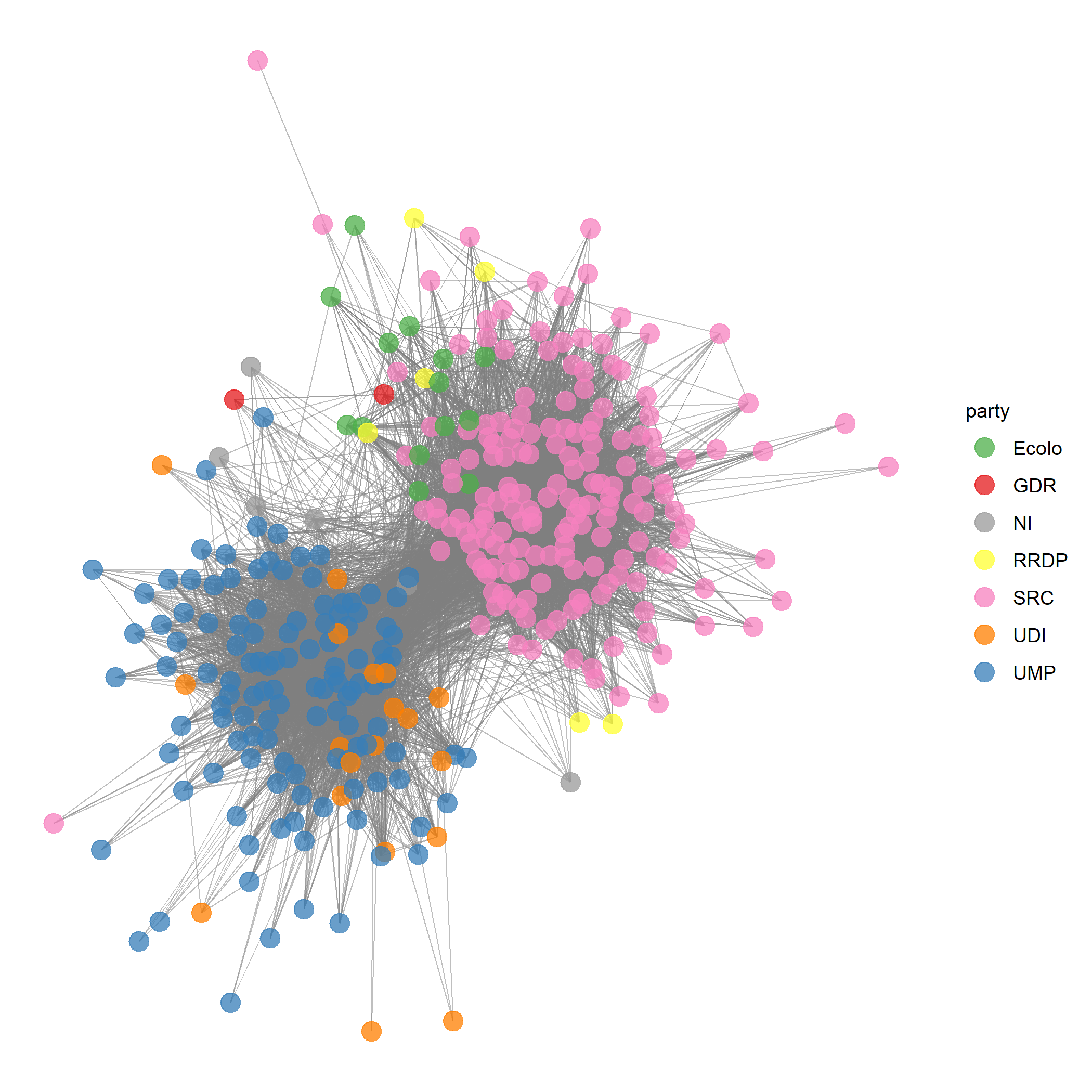
图 4.1: network graphic of french MPs on twitter (p0)
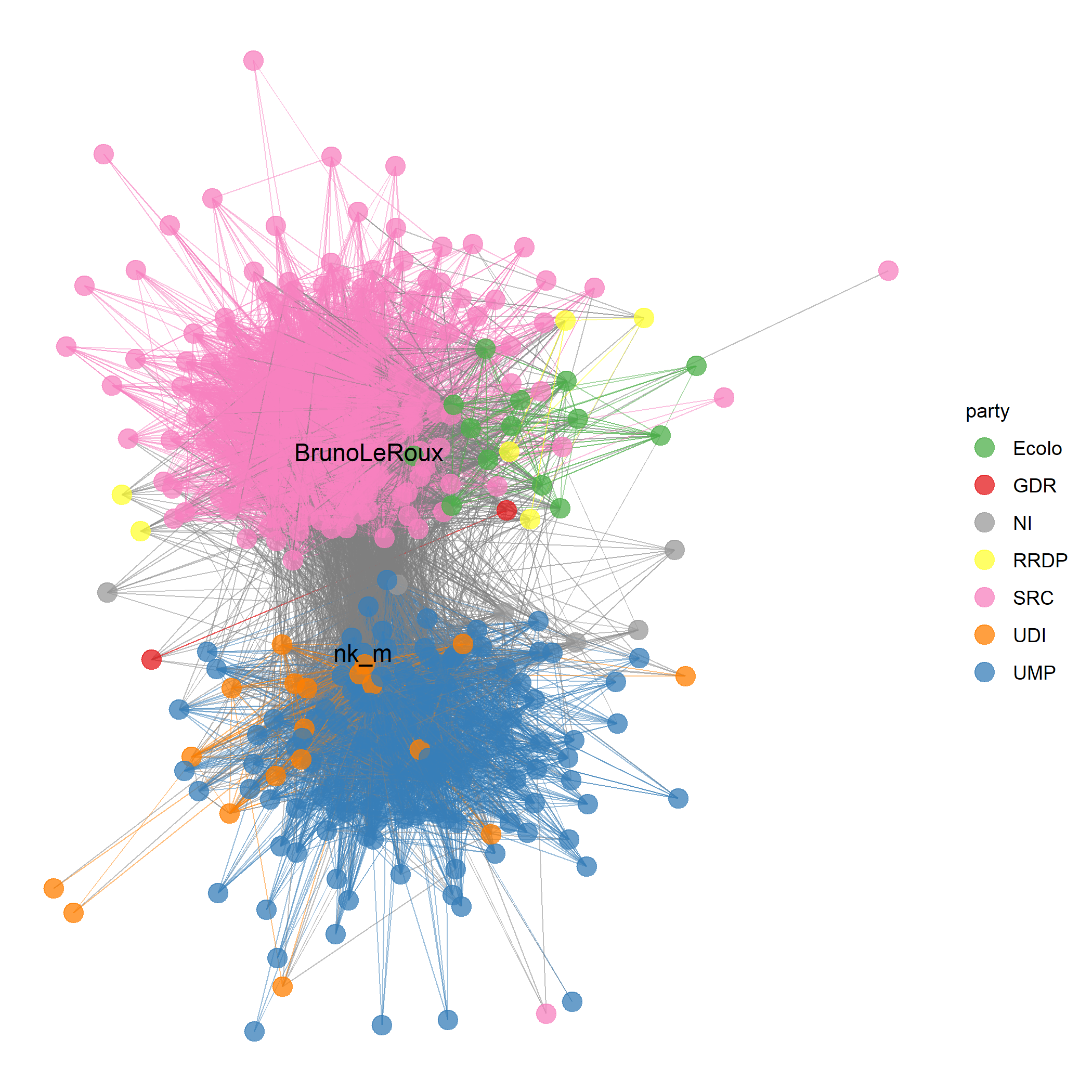
图 4.2: network graphic of french MPs on twitter (p1)
Example (3): Icelandic legal code
# Example (3): Icelandic legal code
source("https://goo.gl/q1JFih")

x = cut_number(as.integer(net %v% "year"), 4)
col = c("#E1AF00", "#EBCC2A", "#78B7C5", "#3B9AB2")
names(col) = levels(x)

p <- ggnet2(net, color = x, color.legend = "period", palette = col,
       edge.alpha = 1/4, edge.size = "weight",
       size = "outdegree", max_size = 4, size.cut = 3,
       legend.size = 12, legend.position = "bottom") +
  coord_equal()

# save plot
ggsave(filename = "pic/network-icelandic.png",
       plot = p,
       device = "png")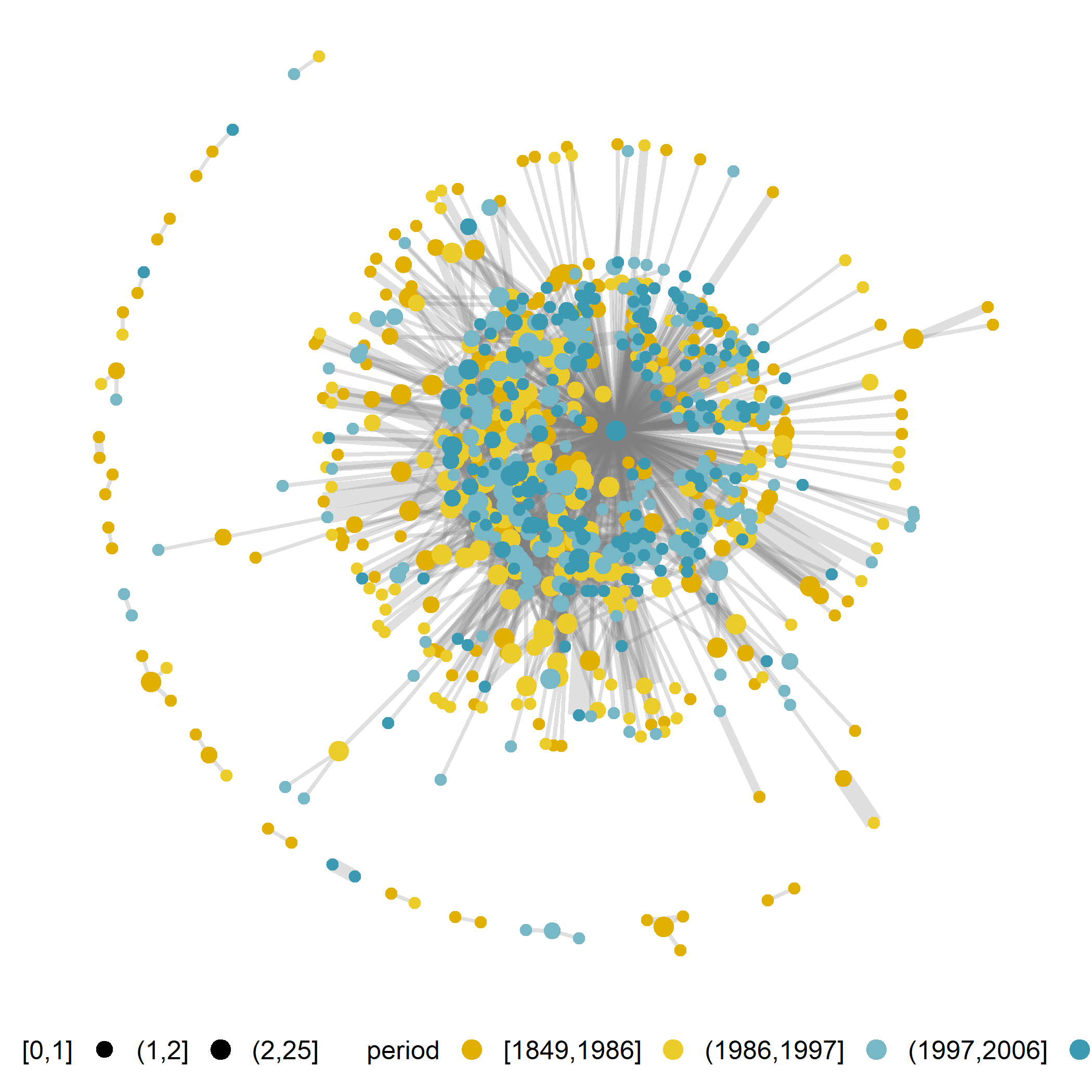
图 4.3: network graphic on icelandic legal
4.4 交互Htmlwidget
4.4.1 使用webshot进行htmlwidget要素截图
R提供了丰富的可视化分析工具,而htmlwidgets包更是将一些炫酷的Javascript包进行封装,提供给R用户进行可视化分析。
然而出了html输出格式对这些htmlwidgets类支持比较完善,其他的输出格式例如pdf或word等并不支持交互的htmlwidgets类要素。
好在webshot包可以将这些动态交互的htmlwidgets类要素进行截图,从而可以实现“阉割版”的可视化输出。
详细的文档说明,可以参看yihui 在bookdown中的官方介绍:HTML widgets。
这里给出一些重要的参数设定参考:
(1)工作区全局性参数设定:
options(
# html widget for xaringan slide
  htmltools.dir.version = FALSE,
  htmltools.preserve.raw = FALSE
  )
(2)R chunk参数全局设定:
knitr::opts_chunk$set(
  # html widget for docx,
  screenshot.force = knitr::pandoc_to("docx"),
  widgetframe_widgets_dir = 'widgets')
(3)特定R chunk代码块参数设定:
``·`{r cpi-show, screenshot.opts = list(selector = ".dataTables_wrapper"), fig.cap="DT table for word output"}
library(DT)
library(webshot)
library(htmlwidgets)
#webshot::install_phantomjs(force = TRUE)
#webshot::is_phantomjs_installed()

DT::datatable(
  cars,
  options = list(pageLength=8,
                 dom="tip")#,

  #height = "100%"
  )
``.`
显然因为.Rmd文件中有部分代码块code chunk不支持MS word输出。有大神指出可以设定htmlwidget的默认行为,例如设定knitr的默认参数(option)为screenshot.force = knitr::pandoc_to("docx")。这样就可以将DT::datatable()之类不支持word输出的,转换为图片格式,从而可输出到word格式。具体可参看:贴文bookdown error when building to word doc
4.4.2 word输出下的yaml设定htmlwidget截图
如果直接在_output.yaml文件中设定MS word输出bookdown::docx_document2,往往会出现如下报错:
Error: Functions that produce HTML output found in document targeting docx output.
Please change the output type of this document to HTML. Alternatively, you can allow
HTML output in non-HTML formats by adding this option to the YAML front-matter of
your rmarkdown file:

  always_allow_html: true

Note however that the HTML output will not be visible in non-HTML formats.

Execution halted

Exited with status 1.因此在yaml区域总是允许html要素呈现的设定总是比较保险的操作:
---
always_allow_html: yes
---
相关讨论和办法可参看:
- “队长问答”剔除的基本的参数设定问题:how to render DT::datatables in a pdf using rmarkdown? 链接。
4.4.3 word输出下的htmlwidget截图区域选定
webshot包的截图定制化功能还是十分强大的。例如pdf或word输出格式下,DT::datatable()的截图,表格最后会有很大的空白行(如图4.4)。
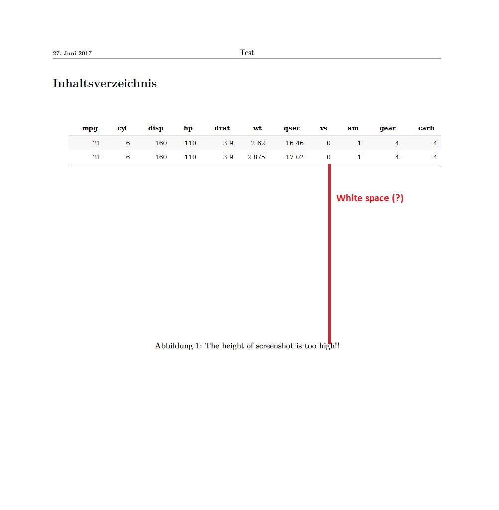
图 4.4: webshot DT table with large margin
相关讨论和办法可参看:
“队长问答”指出的pdf输出下的这个问题:White space from datatable screenshot in Rmarkdown PDF. 链接。
DT包的github讨论贴给出了一些解决线索:knit and webshot.链接。
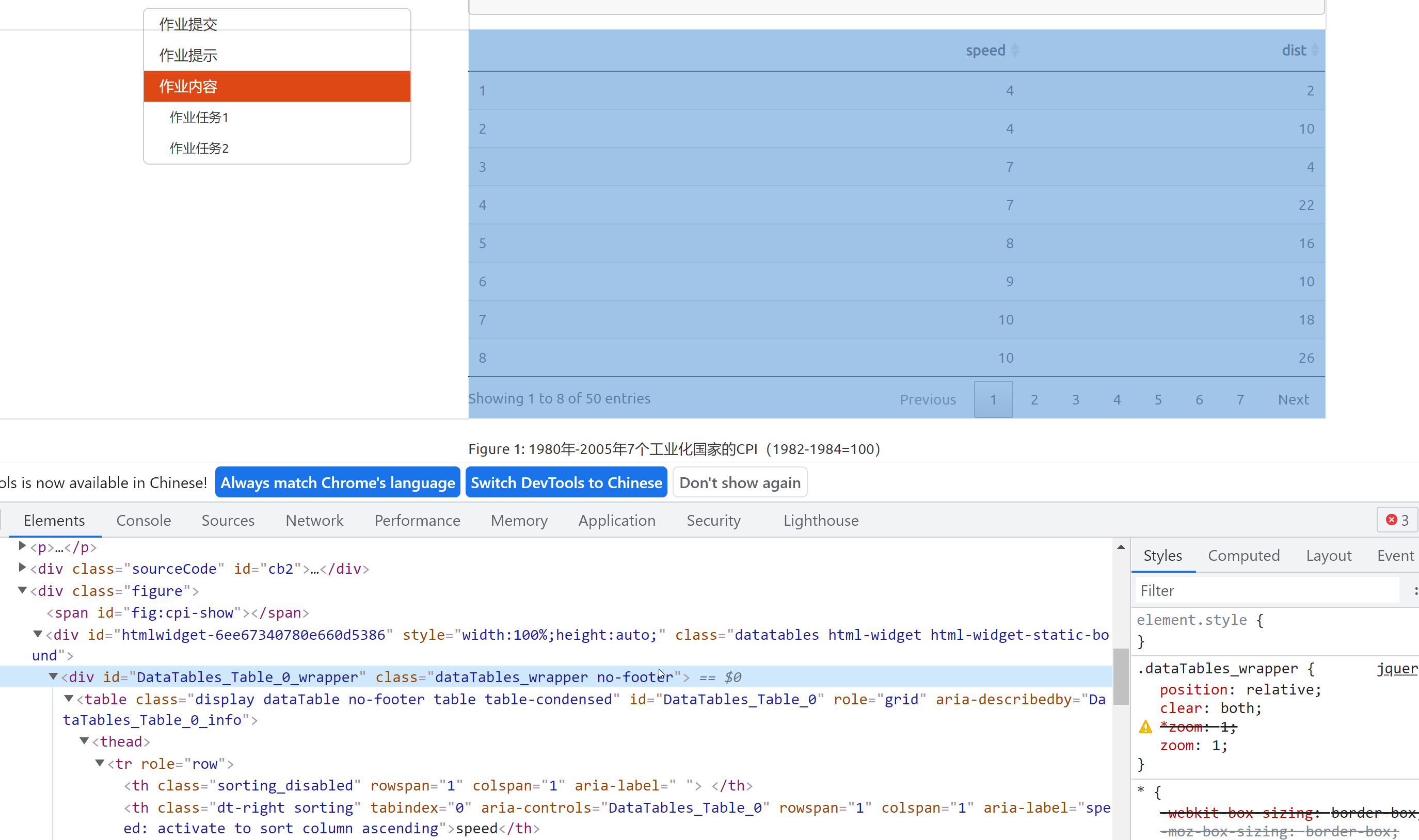
问题的解决办法关键在于参数选项screenshot.opts = list(selector = "css selector")的设定。具体步骤如下:
(1)首先,我们需要读懂webshot(selector = NULL)参数的具体含义(参看官方文档)。简单地说,就是可以通过该参数,根据css规则选定htmlwidget的特定元素,从而实现指定范围的截图。
webshot(url = NULL, file = "webshot.png", vwidth = 992,
  vheight = 744, cliprect = NULL, selector = NULL, expand = NULL,
  delay = 0.2, zoom = 1, eval = NULL, debug = FALSE,
  useragent = NULL)
selector:
One or more CSS selectors specifying a DOM element to set the clipping rectangle to. The screenshot will contain these DOM elements. For a given selector, if it has more than one match, only the first one will be used. This option is not compatible with cliprect. When taking screenshots of multiple URLs, this parameter can also be a list with same length as url with each element of the list containing a vector of CSS selectors to use for the corresponding URL.
(2)然后,我们先使用html_document()直接输出htmlwidget部件(例如上面讨论的DT::datatable()部件),再利用chrome浏览器开发“检查”工具确定要截图的范围和相应的css选择器(selector)。具体见图??:
(3)最后在特定的R代码块上设定相应的CSS参数,例如screenshot.opts = list(selector = ".dataTables_wrapper")。然后再渲染输出为word或pdf格式。
4.4.4 Xaringan突然不显示htmlwidget部件
正常使用Xaringan制作slide,某一天突然报错无法显示DT::datatable()和leaflet等htmlwidgets部件:
WARNING: An illegal reflective access operation has occurred
WARNING: Illegal reflective access by org.apache.poi.util.SAXHelper (file:/D:/r material/Rpackages/xlsxjars/java/poi-ooxml-3.10.1-20140818.jar) to constructor com.sun.org.apache.xerces.internal.util.SecurityManager()
WARNING: Please consider reporting this to the maintainers of org.apache.poi.util.SAXHelper
WARNING: Use --illegal-access=warn to enable warnings of further illegal reflective access operations
WARNING: All illegal access operations will be denied in a future release
widgetframe包的开发者Bhaskar V. Karambelkar专门探讨了相关问题:widgetframe and knitr(见链接)。
初步的解决办法包括:
(1)怀疑是java更新的后果(见讨论)。尝试给java降级! JRE所有版本下载链接在此(见网站)。
(2)如果问题继续出现,怀疑是Rmarkdown进行了调整,背后是pandoc版本进行了升级。具体办法见: xaringan presentation not displaying html widgets(见讨论)。
4.4.5 webshot与knitr::include_graphics()顺次问题
问题描述1:knitr+webshot htmlwidget部件与knitr::include_graphics()代码块先后关系的差异,会导致word输出显示不出来某些图片。
例如(见图4.5):DT_table_A(正常显示图片) \(\rightarrow\) Graph_image_1(不显示图片) \(\rightarrow\) Graph_image_2(正常显示图片)。
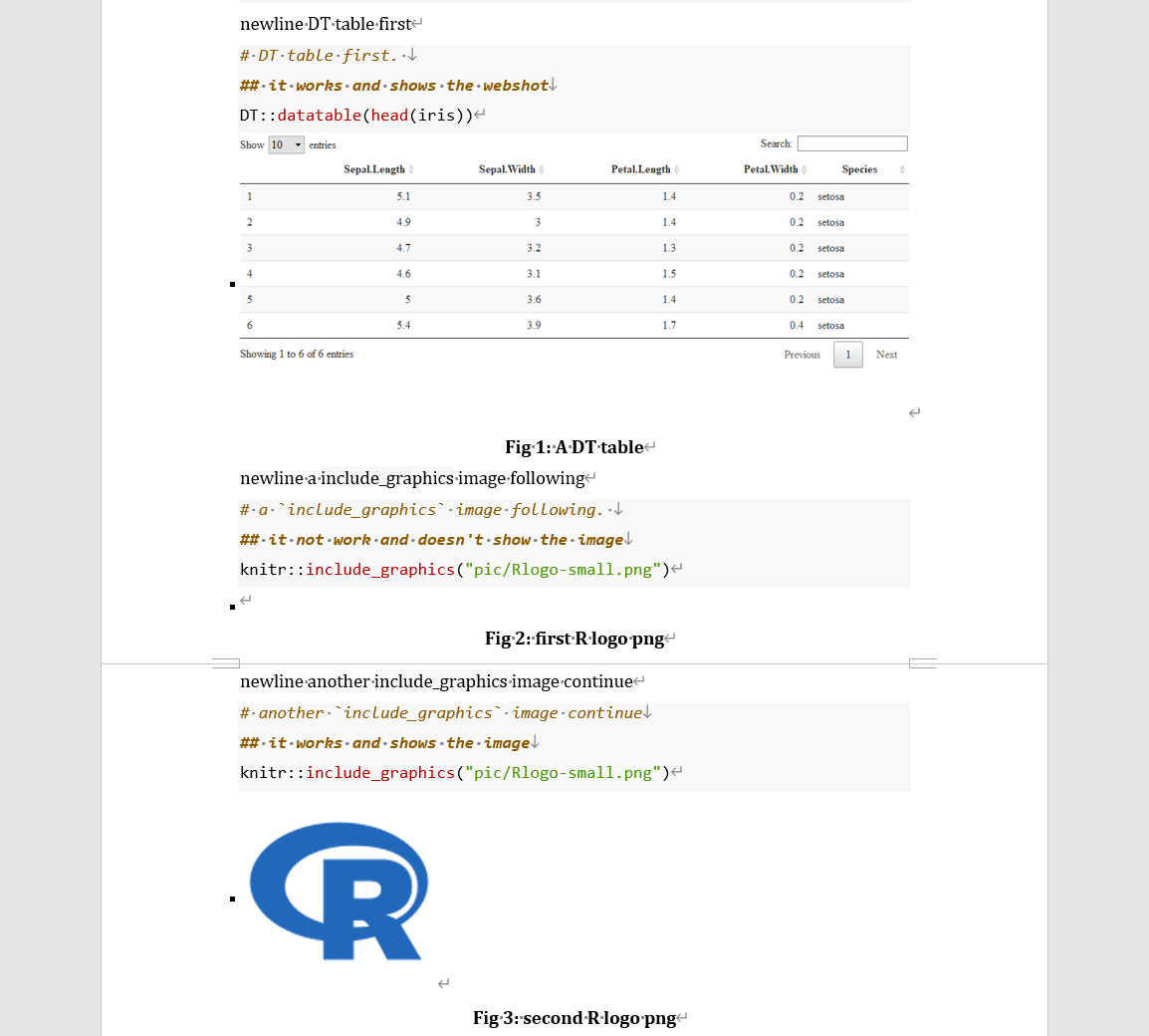
图 4.5: webshot htmlwidget conflict with include_graphics
同样更换两种图片/截图操作的顺次,也会出现类似的问题。例如:Graph_image_1(正常显示图片)\(\rightarrow\) DT_table_A(无法显示图片) \(\rightarrow\) DT_table_B(正常显示图片)\(\rightarrow\) Graph_image_2(正常显示图片)。
上述的执行.Rmd文件代码如下:
---
title: "demo"
output:
  bookdown::word_document2:
    fig_caption: yes
    toc: no
    toc_depth: 4
    number_sections: true
    global_numbering: true
always_allow_html: true
---

newline DT table first

``'`{r check-dataset0, fig.cap="A DT table",screenshot.opts = list(selector = ".dataTables_wrapper")}
# DT table first.
## it works and shows the webshot
DT::datatable(head(iris))
``'`

newline  a `include_graphics` image  following

``'`{r, eval=T, fig.cap= "first R logo png", fig.width=3,fig.height=2}
# a `include_graphics` image following.
## it not work and doesn't show the image
knitr::include_graphics("pic/Rlogo-small.png")
``'`

newline another `include_graphics` image  continue

``'`{r, eval=T, fig.cap= "second R logo png", fig.width=3,fig.height=2}
# another `include_graphics` image continue
## it works and shows the image
knitr::include_graphics("pic/Rlogo-small.png")
``'`
已检查清单:
文档阅读
- yihui’s bookdown book, “2.10 HTML widgets”
环境检查
- pkg安装升级
renv::update(c('bookdown','knitr','webshot','htmlwidgets')) - 浏览器支持
webshot::install_phantomjs(force = TRUE) - 检查支持情况
webshot::is_phantomjs_installed()
- pkg安装升级
.Rmd
yaml参数设定always_allow_html: true。已按要求设置。number_sections: true/false。打开或关闭,问题依旧。global_numbering: true/fale。打开或关闭,问题依旧。
word模板。即便采用默认模板(
word_document2: default或者word_document: default),问题依旧存在。R chunk参数设定:
screenshot.force = TRUE,强制webshot,问题依旧。screenshot.alt = 'path/of/local/webshot_image.png',直接调用本地截图图片,问题依旧。
htmlwidgets::saveWidget()+webshot()。对DT table进行html保存,然后再截图。能正常得到本地截图图片。.Rmd输出为html时(
html_document2:default),DT::datatable()和knitr::include_graphic()的render结果都正常。
R工作环境:
> sessionInfo()
R version 4.1.2 (2021-11-01)
Platform: x86_64-w64-mingw32/x64 (64-bit)
Running under: Windows 10 x64 (build 19043)

Matrix products: default

locale:
[1] LC_COLLATE=Chinese (Simplified)_China.936
[2] LC_CTYPE=Chinese (Simplified)_China.936
[3] LC_MONETARY=Chinese (Simplified)_China.936
[4] LC_NUMERIC=C
[5] LC_TIME=Chinese (Simplified)_China.936

attached base packages:
[1] stats     graphics  grDevices datasets  utils     methods   base

loaded via a namespace (and not attached):
 [1] Rcpp_1.0.7         knitr_1.36         magrittr_2.0.1     here_1.0.1
 [5] rlang_0.4.12       xlsx_0.6.5         fastmap_1.1.0      fansi_0.5.0
 [9] tools_4.1.2        webshot_0.5.2.9002 DT_0.19.1          xfun_0.28
[13] utf8_1.2.2         htmltools_0.5.2    ellipsis_0.3.2     yaml_2.2.1
[17] rprojroot_2.0.2    digest_0.6.28      tibble_3.1.6       lifecycle_1.0.1
[21] bookdown_0.24.3    crayon_1.4.2       zip_2.2.0          rJava_1.0-5
[25] xlsxjars_0.6.1     htmlwidgets_1.5.4  vctrs_0.3.8        glue_1.5.0
[29] evaluate_0.14      rmarkdown_2.11.3   openxlsx_4.2.4     stringi_1.7.5
[33] compiler_4.1.2 pillar_1.6.4 renv_0.14.0 pkgconfig_2.0.3 解决方案1(部分解决):编写代码直接对htmlwidget进行截图,然后再设置代码块chunkscreenshot.alt='pic/webshot/DT-cpi.png',从而调用该截图图片(png、jpeg、pdf)。可参看webshot包问题反馈贴:“Webshot cuts off images with plotly widgets”见链接。
``'`{r webshot, eval=FALSE}
#tempfile = tempfile(pattern = "widgetToPng_", tmpdir ="tempfiles")
name_shot <- "DT-cpi"
filePathHTML = paste0("pic/webshot/",name_shot,".html")
filePathPNG  = paste0("pic/webshot/",name_shot,".png")


htmlwidgets::saveWidget(widget = DT-widget, file = filePathHTML) # at this stage the html is complete

webshot(url = filePathHTML, file = filePathPNG, selector = ".dataTables_wrapper")

# remove html files and dir
dir_rm<- paste0("pic/webshot/",name_shot,"_files")
file.remove(filePathHTML)
unlink(dir_rm, recursive = T)
``'`解决方案2(暂时方案):静态文档输出下(word/pdf等),考虑到knitr+webshot htmlwidget部件的截图呈现,与knitr::include_graphics()代码块图片呈现,存在先后关系上的影响。也即,A类代码运行在前,则A类图片后续都会显示正常,但B类代码的第一项图片会显示不正常,而后续的B类代码的图片又会显示正常。
因此,作为一个暂时解决方案,可以设定一个“虚拟”的第一项B类代码(它会不正常显示,为“隐身”该代码块,可以不设
fig.cap)。
需要注意的是,在html输出下,它会“显身”并正常显示图片!总之,这个只是目前能找到的一个这种办法。后续需要改进!
写在最后:经过经两天的google放狗搜索和反复测试,这个bug始终没有得到解决。基于测试结果,先后次序上的问题,让人感觉好像是numbering自动序号的嫌疑。不知道是不是bookdown包的锅,或者是knitr的锅。